
-
 Kevin Yu
- 02 May, 2020
Start Your Cloud Computing Journey with Colab
Cloud computing is a term used to describe the use of hardware and software delivered via network (usually the Internet). The term comes from the use …
In the previous post , we have walked through the basics of using Google Colab . In this article, we will be doing an experiment on training a custom object detection model on the Cloud ! Let’s get started.
In this experiment, the custom object detection model will be trained based on a YOLOv3-tiny Darknet Weight. If you have never tried Yolov3 Object Detector, you may visit my previous YOLOV3 post , or you may visit the YOLOV3 site for more information.
Yolov3 Dataloader (Google Colab) V2 is tailored for those who want to train their custom dataset on a Yolov3-tiny Model. I have not tested it with the normal Yolov3 weight, but feel free to try modifying the parameters in the config file. If you following the instructions in the Notebook step by step and run every cell accordingly, it will generate a new trained-weight in the end, and you may download it from Colab to your local machine. The reason why I configured this training with YOLOv3-tiny is that it is much easier to deploy it to the Edge devices such as Raspberry Pi and Jetson Nano. In this experiment, I deployed it on my Jetson AGX Xavier with satisfactory outputs.
I wrote a Jupyter Notebook for training. You may download it directly with the LINK, and you may clone it with my repo .
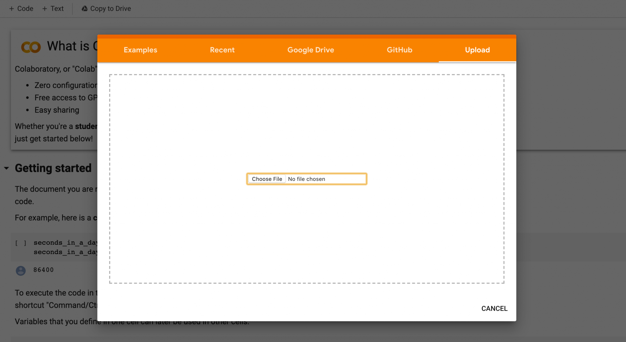
Upload it to Colab
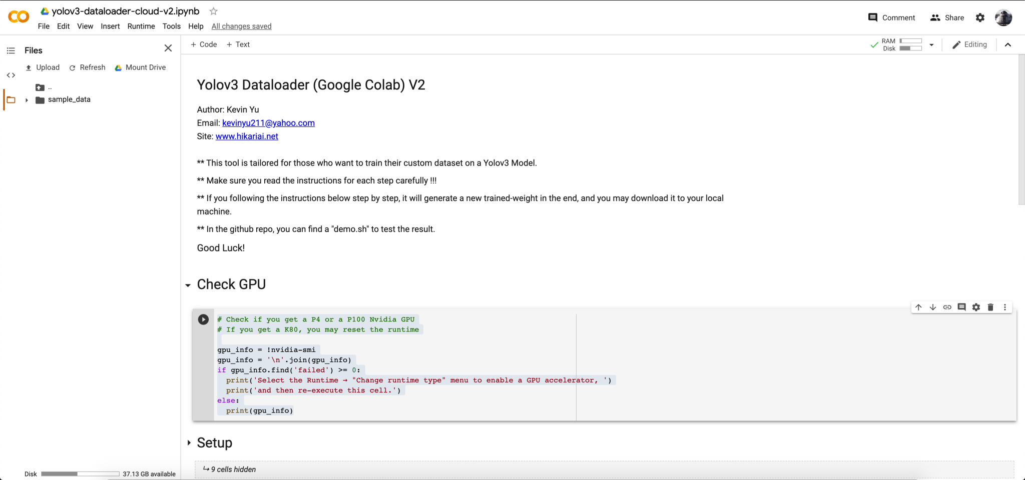
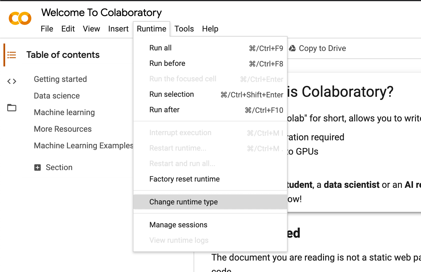
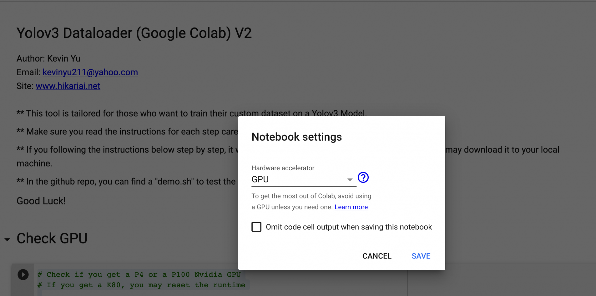
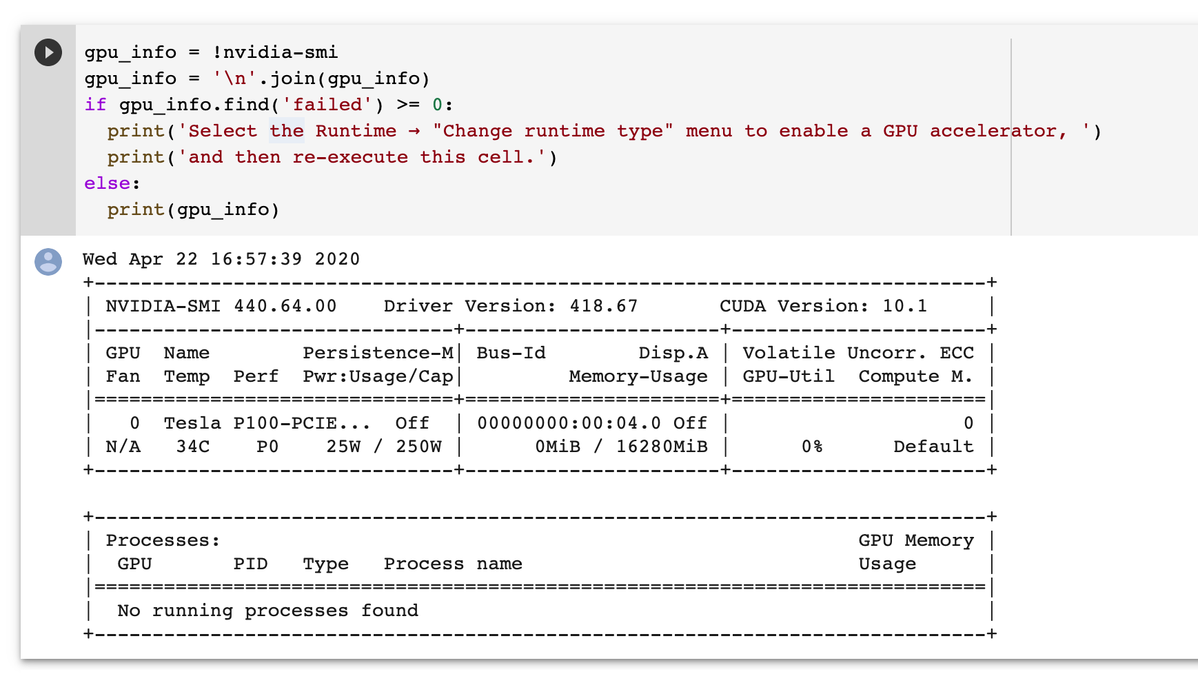
I wrote a Python script for checking if you receive a P100 or a T4 GPU in your runtime. Simply copy and paste the scripts below to the cell and run it. If you do not get a P100 or a T4, then you may go to the Menu bar, and find Runtime » Factory rest runtime, and your Colab VM will be re-initialized.
 1# Check if you get a P4 or a P100 Nvidia GPU
 2# If you get a K80, you may reset the runtime
 3
 4gpu_info = !nvidia-smi
 5gpu_info = '\n'.join(gpu_info)
 6if gpu_info.find('failed') >= 0:
 7  print('Select the Runtime → "Change runtime type" menu to enable a GPU accelerator, ')
 8  print('and then re-execute this cell.')
 9else:
10  print(gpu_info)
I used a tool called LabelImg to label all my images for training. You may check out a good tutorial on how to make your dataset with LabelImg HERE. The labeling process is somewhat tedious, but it is a must for training a custom dataset.
You may use the commands below to download LabelImg on Ubuntu 18.04. If you are a windows user, you may check out the installation guide HERE.
1$ sudo apt-get install pyqt4-dev-tools
2$ sudo apt-get install python-lxml
3$ sudo apt-get install python-qt4
4$ sudo apt install libcanberra-gtk-module libcanberra-gtk3-module
5$ git clone https://github.com/tzutalin/labelImg.git
6$ cd labelImg
7$ make qt4py2
8$ python labelImg.py
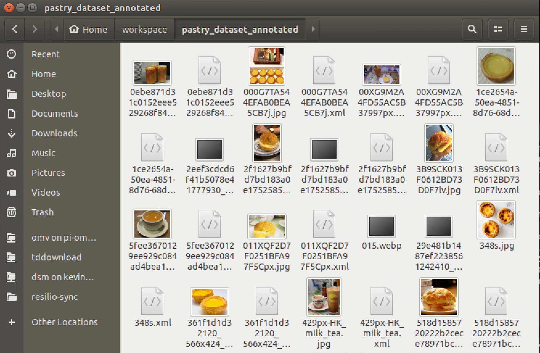
By the end of the labeling process, your dataset folder should look something as shown below.
Each image should have one .xml file with it, and both the image and the .xml file have the same name.
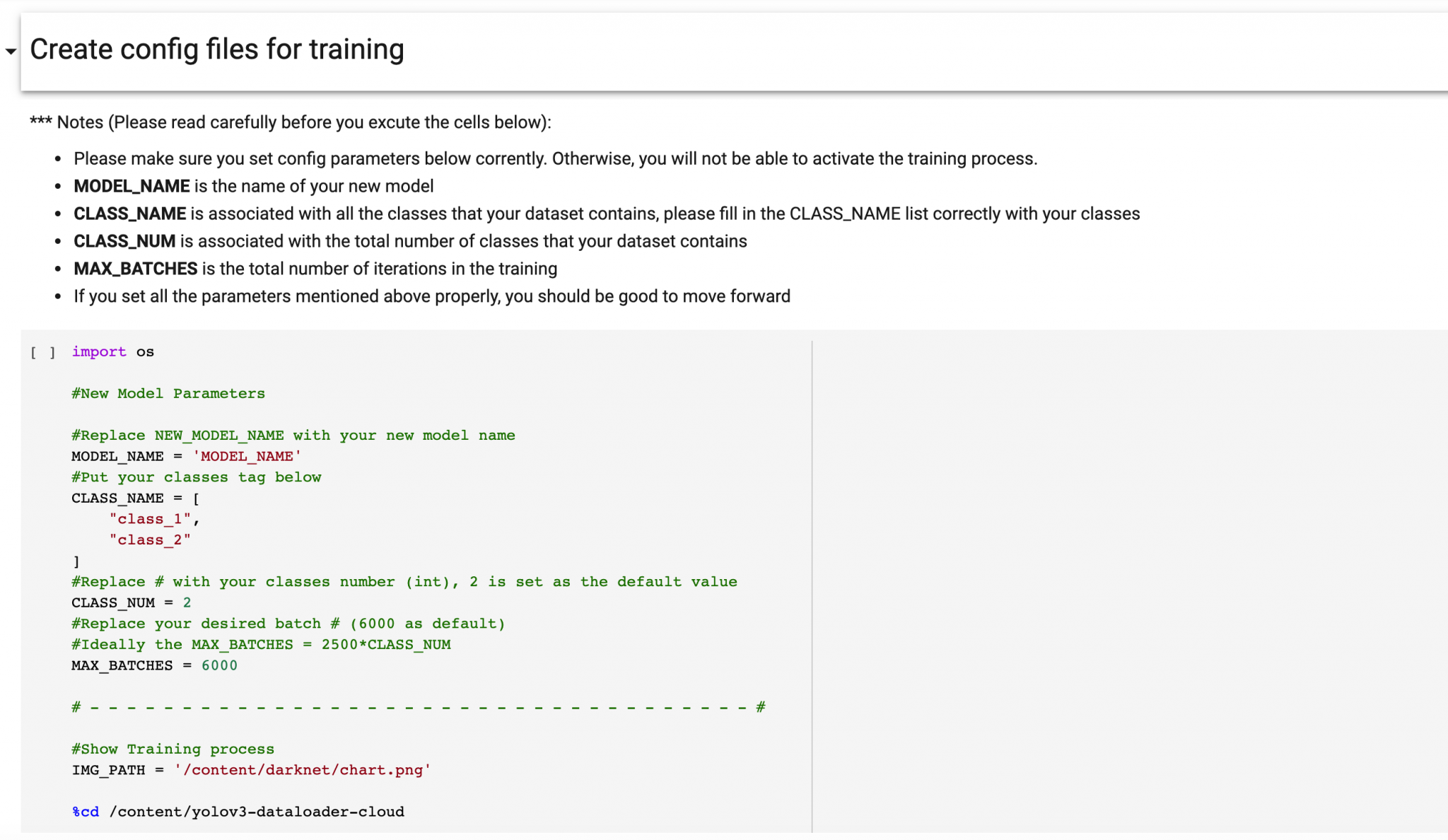
The step is the most important step for in entire training process. If you mess it up, you might not get a good output weight as expected.
You need to update FOUR parameters before initializing the training process. MODEL_NAME, CLASS_NAME, CLASS_NUM, and MAX_BATCHES. You may find the descriptions for these four parameters in the Notebook as shown below.
Go through the steps, and run each cell exactly once. If you are doing all steps correctly, your file structure should like something as shown below:
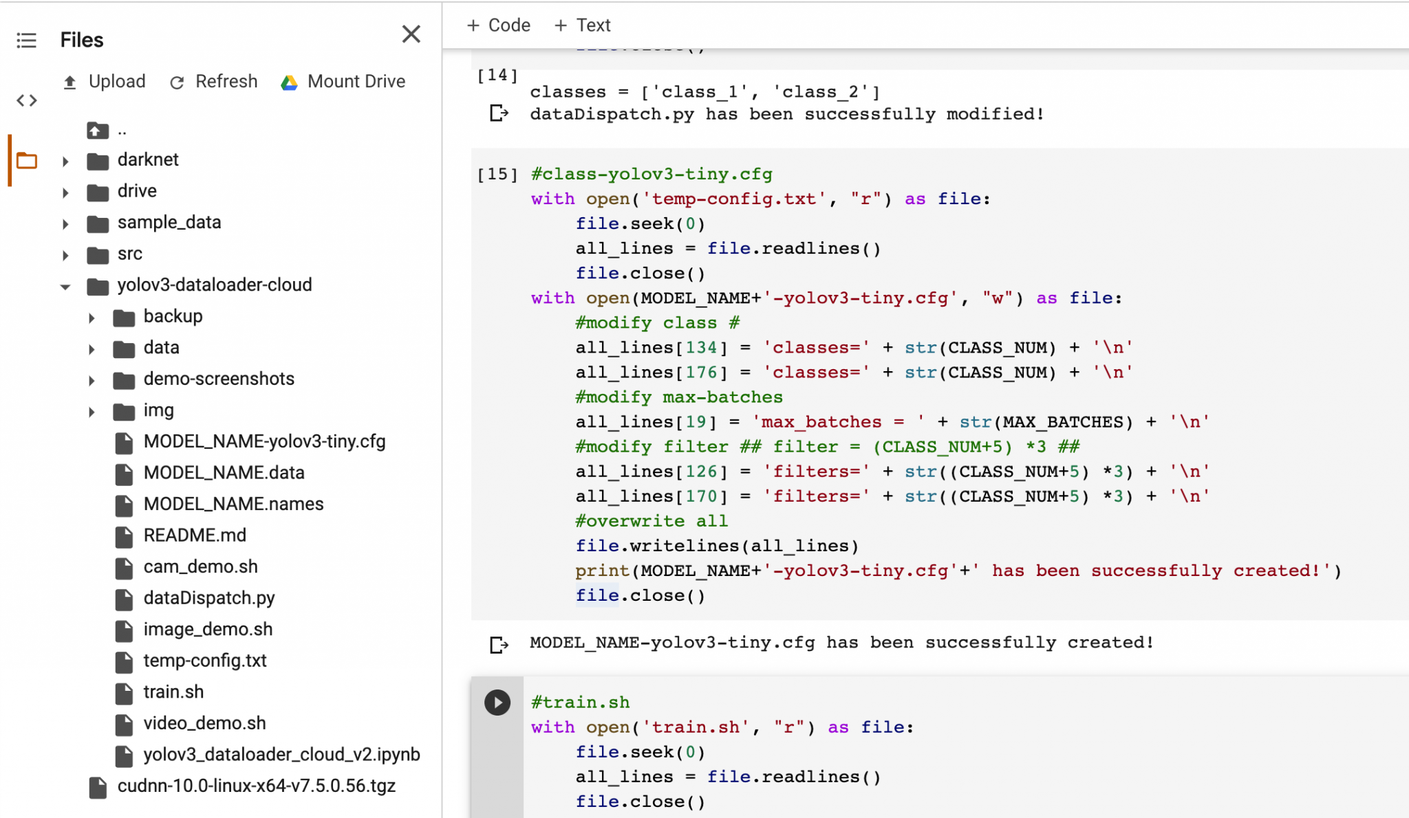
Notes: the MODEL_NAME is the default name in the config, you need to update the parameters based on your own preference.
Check if the directory contains the .data, the .names, and the .cfg files. If you miss one or more of the files, please check the instructions from the above steps.
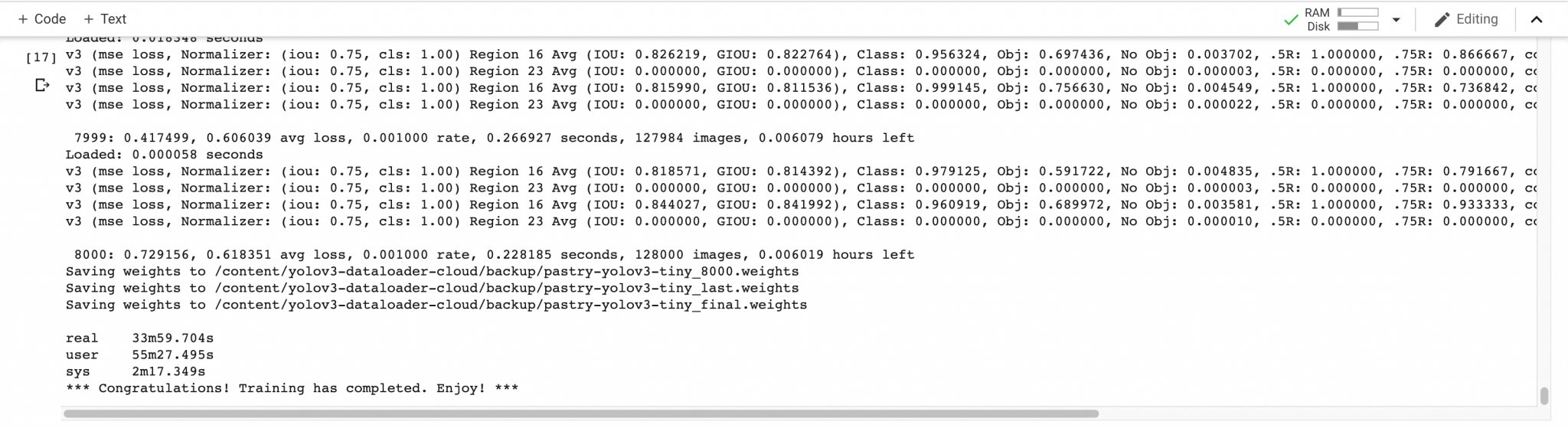
Once the training process starts, you should have a similar output as shown below:
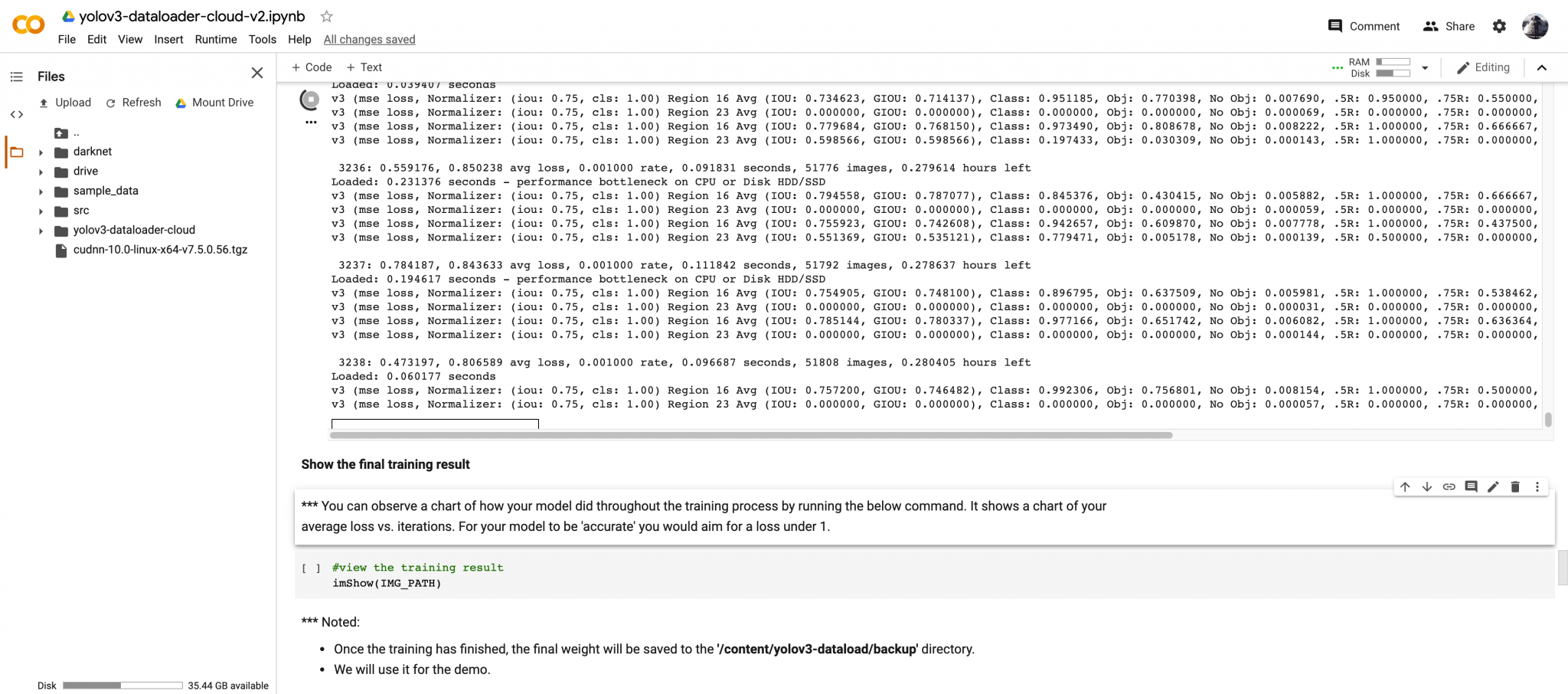
The total training time with my Pastry model (contains 200 images) takes roughly 30 minutes with a P100 GPU. However, it takes more than an hour on my Xavier to finish the training. As you can tell, the P100 is a costly but very powerful GPU for Deep Learning
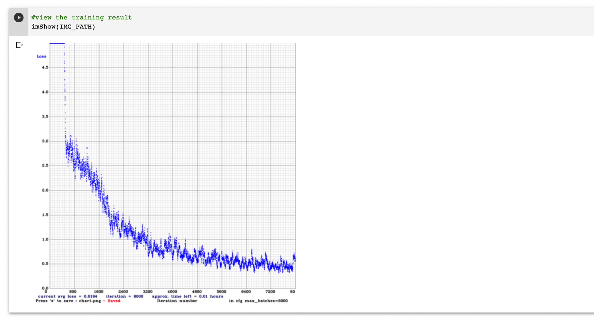
You can observe a chart of how your model did throughout the training process by running the below command. It shows a chart of your average loss vs. iterations. For your model to be ‘accurate’ you would aim for a loss under 1.
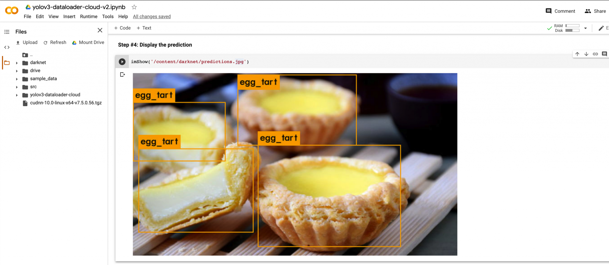
Once the training has finished, the final weight will be saved to the /content/yolov3-dataload/backup directory.
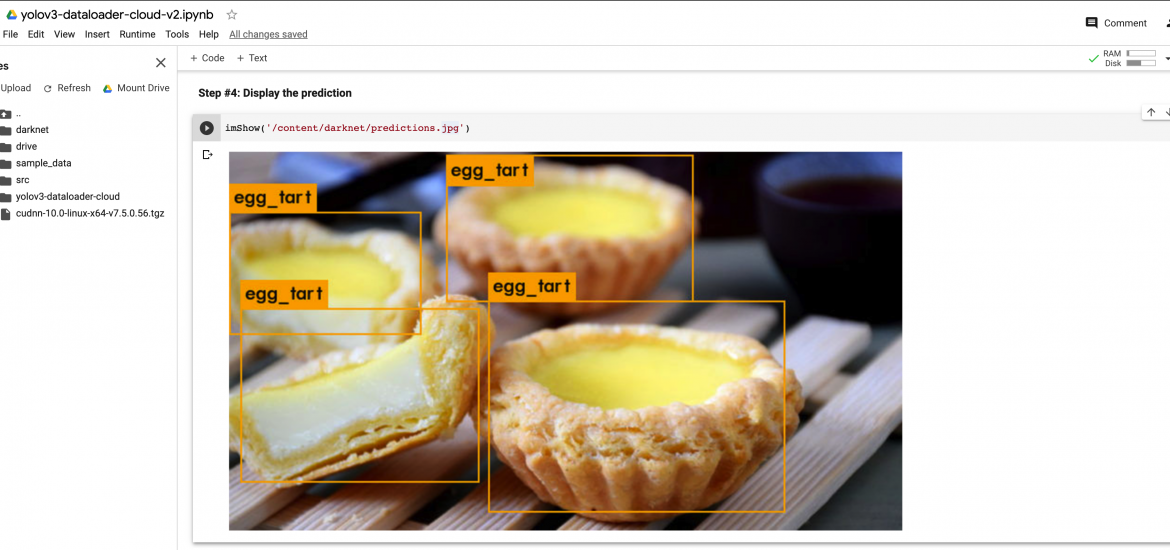
Image Input
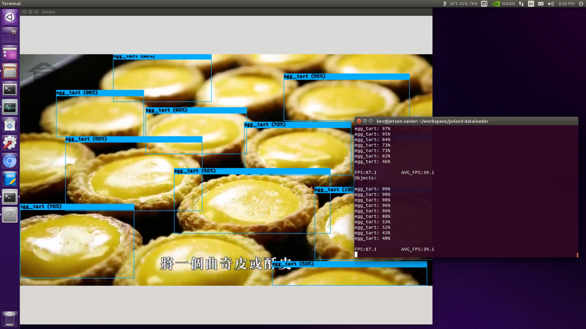
Video Input
With this YOLOv3-Dataloader tool, you may easily train your own YOLOv3-tiny Object Detection Model on the Cloud, and it is TOTALLY FREE. If you encounter a disconnection issue, you may just hit the Reconnect button, your data will not lose, and the training process should not be terminated unless you manually restart the runtime. For one-time usage, Colab allows you to activate a runtime for a continuous 12-hour usage, and it is good enough for a normal training process. I hope you could find something useful in this post. Happy training !
Written By
In the upcoming months and years, I want to help make learning Machine Learning and Cloud Computing topics easier by writing lots of articles showing of practice cases on Cloud and Edge devices. Furthermore, I’m planning on creating an AI and Cloud …
Cloud computing is a term used to describe the use of hardware and software delivered via network (usually the Internet). The term comes from the use …
In the summer of 2022, I decided that it was time to try again to learn a bit about Kubernetes because it’s something that becomes more and more …